Part 1: Why do we care about scaling?
1.1 The promise(?) of foundation models for biology
In just a few years, foundation models have become an everyday part of how many of us work. We ask a chatbot to explain a paper, plan and implement an analysis pipeline, check our results against the current literature, and suggest the next hypothesis to test. Behind all of these tasks is the same underlying model, with some extra training on top and access to tools like web search and code execution. That’s the core idea behind a foundation model: train one large model on a huge amount of broad data, then reuse it for many different tasks, instead of building a new model from scratch each time.1
Biology has had a few of these moments too, where a single model changed what the field thought was possible. The clearest is AlphaFold. Predicting a protein’s 3D structure from its amino acid sequence had resisted decades of work, and in 2020 AlphaFold began producing predictions that were often close to experimental accuracy.2 Its creators shared the 2024 Nobel Prize in Chemistry.3 More recently, AlphaGenome reads up to a million letters of DNA and predicts, in a single model, how a change in that sequence affects gene expression, splicing, and chromatin accessibility across many cell types.4 (Strictly speaking, neither is a foundation model in the usual sense, but both show what large models trained on biological data can do.)
So it’s natural to wonder whether we can borrow this success story from computer science for other kinds of biological data, like single-cell and multiomic measurements, where large atlases now span millions of cells. Before we do, though, two questions are worth pausing on. The first is what we actually want a foundation model in biology to do. “A model that understands cells” is inspiring but vague, and the answer shapes what data we train on and how we judge success. Researchers closer to the biology have written thoughtfully about this, and the perspective by Bunne et al. on building an AI virtual cell is a great place to start.5 The second question, and the focus of this post, is how we should think about scaling. It’s tempting to picture scaling as buying more GPUs or collecting more data, but those are only part of the story.
In Part 1, I’ll build up the intuition and evidence for why scaling works at all. In Part 2, I’ll walk through what it takes in practice.
1.2 More data, bigger models
Let’s start with something familiar. In an experiment, the more samples we collect, the more precise our estimate: the standard error of a mean shrinks roughly like \(1/\sqrt{n}\). Each extra sample helps a little less than the one before, but on a log scale the pattern is perfectly steady: every tenfold increase in samples cuts the error by the same factor, about three. Plotted on log-log axes, that’s a straight line, and as we’ll see in Section 1.3, it’s exactly what scaling laws look like.
Precision is only half the story, though. A model can only learn what it is flexible enough to express. Fit a straight line to data that curve, and more samples just make us more confident about the wrong line. The error that comes from the model’s shape doesn’t shrink, no matter how much data we add. And biological data are rarely straight lines. Cells moving through development or responding to pathology trace out complicated, curved paths in gene expression space (what mathematicians call a manifold), and capturing that takes a more flexible model, which in practice means more parameters.
However, we also know that with too little data, a flexible model has enough freedom to fit the noise along with the signal. The fit will look great on the data it was trained on but will do poorly on new data (this is called overfitting). More data is what keeps a flexible model honest: with enough samples, the noise averages out, and the extra flexibility goes toward the real structure.
In other words, data and model size go hand in hand. More data lets us afford a bigger model, and a bigger model lets us get more out of the data. Grow only one and we eventually hit a wall: either the model is too simple to use the extra data, or there isn’t enough data to support the extra parameters.
This is the intuition behind scaling laws: they describe how fast performance improves as we grow data and model size, and how to balance the two.
For the curious. Classical statistics pictures this as a U-shaped curve: error on new data first falls as the model gets more flexible, then rises once it starts overfitting. Modern deep learning brought a surprise. Very large models, with far more parameters than data points, often generalize well anyway, a phenomenon called “double descent.” Overfitting is still real, but where the wall sits turns out to be more subtle than the textbook picture suggests.
1.2’ Same story but with a theoretical view: A VC-dimension view
Section 1.2 left us with a balancing act: flexible models need enough data to stay honest. Statistical learning theory gives us a way to make that idea a bit more precise, through something called the VC dimension, after Vladimir Vapnik and Alexey Chervonenkis.6
The idea is to measure a model’s flexibility by asking how many data points it can fit no matter how they’re labeled. Take a straight line used to separate two groups of points on a page. Give it any three points (not all in a row), color them however you like, and some line can always split the colors apart. With four points, that breaks down: put two red and two blue at opposite corners of a square, and no single line can separate them. So the VC dimension of a line on a page is three. In general it grows with the number of things the model can adjust, roughly its number of parameters.
Why does this matter? If a model is flexible enough to fit any labeling of our data, then fitting our data perfectly tells us nothing, because it would have fit random labels just as well. Learning only means something when the data outnumber the model’s flexibility. Biologists already know a version of this: a regression with as many variables as samples fits perfectly and means nothing, which is why clinical prediction models follow rules of thumb like “about ten events per variable.”7
The theory turns this into a rough rule. The gap between how well a model does on its training data and on new data shrinks roughly like
\[\sqrt{\frac{d}{n}},\]where \(d\) is the VC dimension and \(n\) is the number of samples. Two things fall out of this. First, the \(1/\sqrt{n}\) from Section 1.2 is back: more data still helps in a steady, log-log-straight way. Second, to keep the gap fixed as the model grows, the data have to grow along with it. That’s “data and model size go hand in hand,” now with a formula attached.
Like any formula, this one comes with assumptions, and two of them matter a lot for biology. First, it assumes our samples are independent draws from the same population we’ll later apply the model to. In single-cell data that’s rarely true: cells from the same donor, tissue, or batch share a lot, so a hundred thousand cells from one donor are not a hundred thousand independent looks at human biology. The effective \(n\) can be much smaller than the number of cells, a thread we’ll pick up in Section 2.3. Second, it only promises that the model will do about as well on new data as on its training data, for the same task it was trained on. It says nothing about downstream tasks, like annotating cell types or predicting perturbation responses, which are usually what we actually care about. Even in computer science, the cleanest scaling laws are for the pretraining loss (how well the model predicts held-out text). Downstream performance is much noisier: it can stay flat for a while and then jump,8 and how smooth it looks depends partly on how we choose to measure it.9 We’ll come back to this in Section 2.3.
There’s also a catch in the other direction, and it’s a good one. VC bounds describe the worst case, and for modern neural networks they are far too pessimistic. Large networks can memorize completely random labels,10 so by this measure they should overfit badly, yet on real data they often generalize well (the double descent surprise from Section 1.2). Theory gives us the right intuition about the trade-off, but it can’t tell us the actual numbers for a given model and dataset. To get those, we measure them, and that’s what scaling laws do.
1.3 Scaling laws: an empirical surprise
Section 1.2’ ended on a puzzle. Worst-case theory says huge neural networks should overfit, yet in practice they keep getting better as they grow. Earlier work had hinted that this improvement is predictable,11 and in 2020 Kaplan and colleagues at OpenAI showed it cleanly: as they grew model size, data, and compute, the loss fell along a straight line on log-log axes, a power law, across more than seven orders of magnitude.12
What makes this useful is prediction. With careful experimental design (here, the experiments are on models rather than on cells), we can run a series of small, cheap training runs, fit the curve, and estimate how a model will do on a budget many times larger. Just as in the lab, “careful” means controlling the right variables. Chinchilla shows how to balance model size against data for a given budget,13 and μP shows how to choose hyperparameters, like the learning rate, so that what we learn on small models carries over to big ones.14
To see what such an experiment looks like, take Chinchilla. Training cost is measured in compute, counted in FLOPs (floating-point operations, the individual multiplications and additions a computer performs). A handy rule of thumb is that compute is about 6 × (number of parameters) × (number of training tokens), where a token is one unit of input: a word piece in text or, in many single-cell models, a gene. So for a model of a given size, compute grows in direct proportion to the data: train on twice as many tokens, and it costs twice as much. That means a fixed compute budget forces a trade-off. A bigger model can only see less data, and a smaller one can see more. It’s a lot like a fixed sequencing budget, where we choose between sequencing more cells shallowly or fewer cells deeply. Hoffmann and colleagues trained over 400 models in all, and in one set of experiments they held the compute budget fixed and traded model size against data, at several budgets (Figure 1). Each budget traces a U-shaped valley: too small a model can’t make use of the data, and too big a model doesn’t get to see enough of it, the same balance as in Section 1.2. The bottom of each valley is the best split for that budget, and following those bottoms as the budget grows tells us how to scale up.
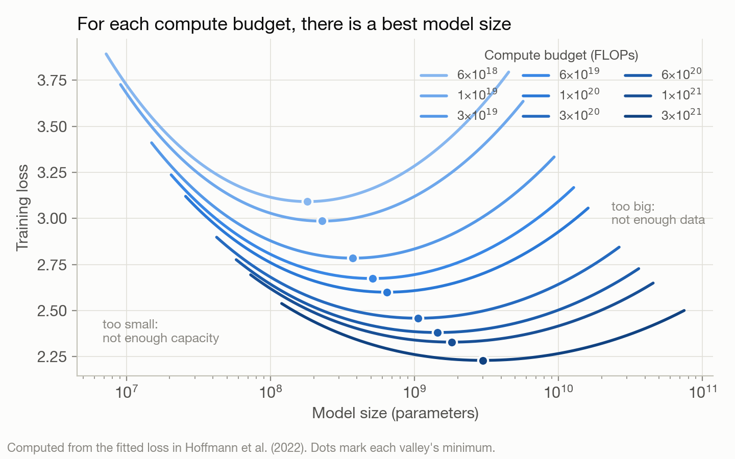 Figure 1. For each fixed compute budget, there is a best model size: too small and the model can’t use the data, too big and it doesn’t see enough of it. Computed from the fitted loss in Hoffmann et al. (2022); adapted from their Figure 3.
The second experiment is about hyperparameters, the settings we choose before training. Some describe the model’s shape, like its width (how big each layer is) and depth (how many layers it has). Others describe how it’s trained, like the learning rate, which sets how big a step the model takes each time it updates. Shape turns out to be fairly forgiving: Kaplan et al. found that, for a given number of parameters, performance depends only weakly on the exact width and depth. The learning rate is trickier. It changes over the course of training according to a schedule, and its best value depends on other settings, especially the batch size (how many examples the model sees per update). The traditional approach was to tune these separately for each model: try a range of values and keep the best. That works for small models, but it gets expensive fast, because every trial on a big model is a full training run, and it doesn’t tell us what to use at a scale we haven’t tried yet. The newer approach treats the hyperparameters themselves as something that scales. At each of several small budgets, we sweep the learning rate and find the best value (Figure 2a), then fit how that best value changes with the budget (Figure 2b). The DeepSeek team, for example, did this for budgets from \(10^{17}\) to \(2 \times 10^{19}\) FLOPs and found that the best learning rate falls, and the best batch size grows, as smooth power laws of compute. A check at \(10^{20}\) FLOPs confirmed that the predicted settings still worked well.15 μP takes a complementary route: it changes how the network is set up so that the best learning rate barely moves as the model gets wider, so a value tuned on a small model can be carried straight over to a large one. Either way, the goal is the same: every point on the scaling curve is fairly tuned, so we’re measuring the effect of scale, not the effect of tuning.
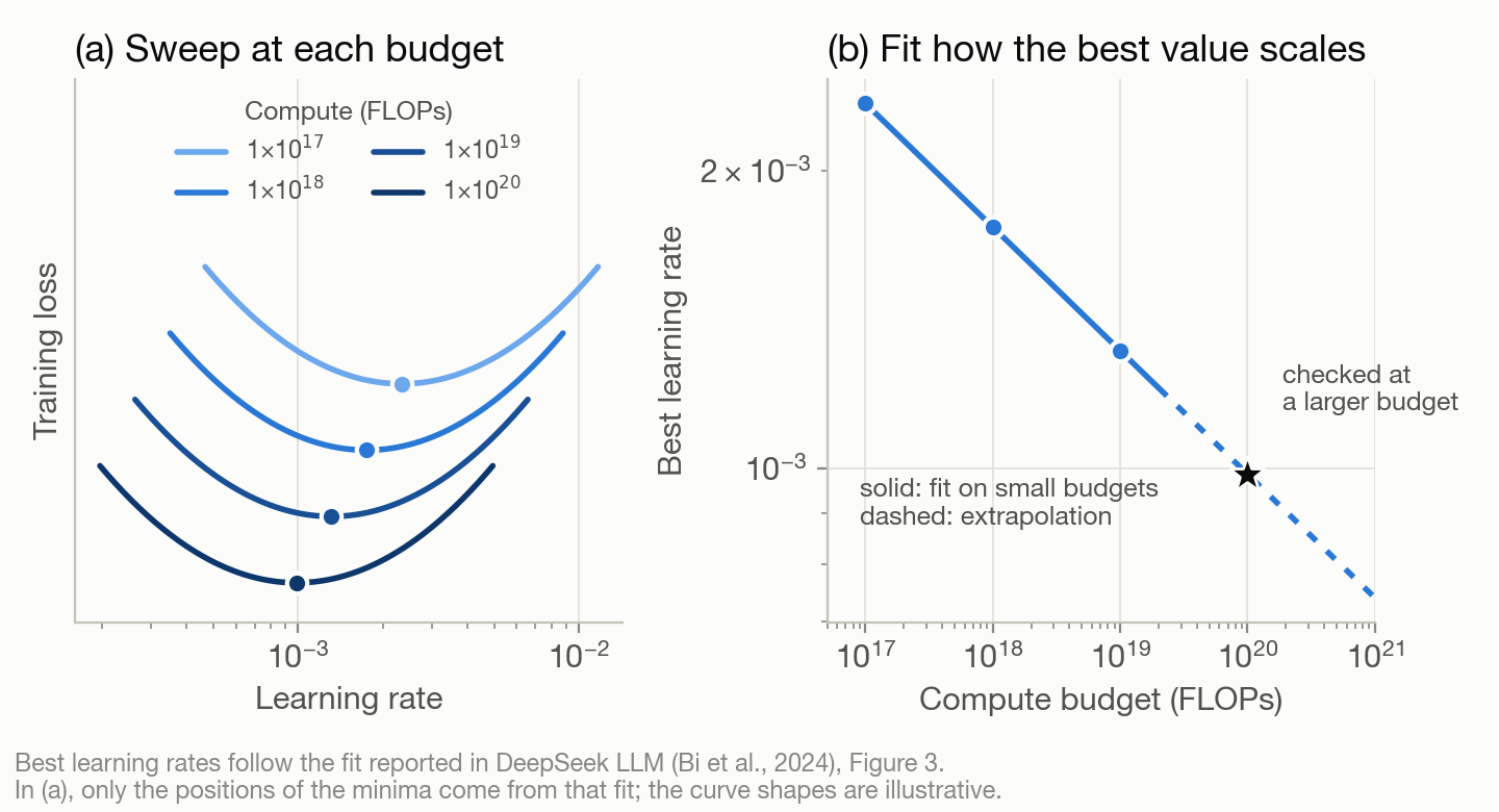 Figure 2. (a) At each budget, we sweep the learning rate and find the best value. (b) The best value follows a power law in compute, so a fit on small budgets predicts the right setting for a larger one. Best learning rates follow the fit in Bi et al. (2024), Figure 3; the curve shapes in (a) are illustrative.
Together, they let us compare design choices at small scale, such as two architectures or two ways of representing a cell, and pick the most promising one before committing a large budget to it. This kind of experimental design is still rare for foundation models in biology. So it’s worth testing whether these ideas hold for biological data. Below, I explain several steps that may be helpful for realizing these experiments.
For the curious. Chinchilla fits the loss with a formula that echoes Section 1.2:
\[L(N, D) = E + \frac{A}{N^{\alpha}} + \frac{B}{D^{\beta}}\]Here \(N\) is the number of parameters and \(D\) is the number of training tokens. \(E\) is the loss no model can beat (the randomness inherent in the data). \(A/N^{\alpha}\) is the penalty for a model that is too small, and \(B/D^{\beta}\) is the penalty for too little data. Their fitted values were \(E = 1.69\), \(A = 406.4\), \(B = 410.7\), \(\alpha = 0.34\) and \(\beta = 0.28\). Each penalty is a power law, which is why it appears as a straight line on log-log axes.
Following the bottoms of the valleys in Figure 1, Chinchilla found that model size and data should grow at about the same rate as compute grows. Kaplan et al. had concluded that the model should grow much faster than the data (Figure 3). Much of that difference comes from how the runs were set up: Kaplan’s team used the same learning-rate schedule for every run, no matter how long it trained. Hoffmann et al. point out that this made the loss of shorter training runs look worse than it really was, which pushed Kaplan’s conclusion toward growing the model faster than the data. For the details, see Hoffmann et al. (2022), especially their Figure A1 on the length of the learning-rate schedule.
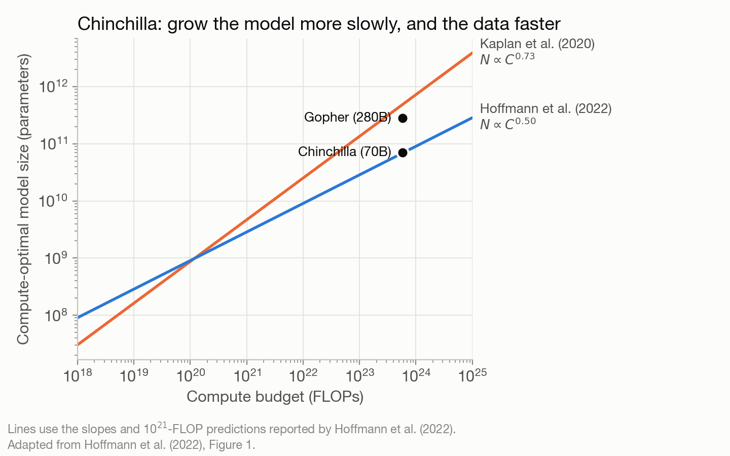 Figure 3. As compute grows, Chinchilla’s analysis says to grow the model more slowly (and the data faster) than Kaplan et al. suggested. Adapted from Hoffmann et al. (2022), Figure 1.
Part 2: There’s more to scaling than more GPUs
Part 1 ended on a hopeful note for language models: with carefully designed experiments on small budgets, we can predict how a much bigger model will do. What we don’t know yet is whether biology has the same success story. Finding out (in my case, with single-cell multiomic data) takes more than getting more GPUs. Every point on a scaling curve is a trained model, and the curve is only as trustworthy as the experiments behind it. Three things help make those experiments work. First, we need to record exactly which model architecture, which hyperparameters, and which data went into each training run, so that our comparisons are fair and any result can be traced back and reproduced (Section 2.1). Second, we need to make sure we’re using our resources well, from loading the data to keeping the GPUs busy, because wasted compute means fewer experiments and slower answers (Section 2.2). Finally, we need to think about how to evaluate the results, because a lower training loss doesn’t automatically mean a model has learned more biology (Section 2.3).
2.1 Experiments: can we trust our comparisons?
A single scaling study can easily involve hundreds of training runs. Each one uses a particular model architecture, a particular set of hyperparameters, and a particular slice of the data, and each one becomes a single point on a curve. If we lose track of what went into any of those points, we can no longer tell whether a difference between two runs comes from scale or from something we changed by accident.
At the Allen Institute, my manager brought in a software engineer to help our team build good habits for exactly this. The core idea is to separate two kinds of code. The library is the reusable part: the model, the data processing, the training loop. The runner is the thin layer on top that launches a specific experiment. The library changes slowly and carefully. The runner is where we say “train this version of the model, at this size, on this data, with these settings.”
The software engineer gave us a set of guidelines, including best practices for working with Claude as a coding assistant (reusable skills and agents). But a guideline isn’t a design. Our multiomic foundation model is complex, and turning those guidelines into a working training pipeline took many decisions that fell to me as the ML scientist on the project. For example, how should the code and configs be organized so that the model stays modular, letting us swap in a different encoder architecture for one modality, or a different method for fusing modalities together, without rewriting anything? And on the infrastructure side, should we train with a library like DeepSpeed (more on that in Section 2.2)? I may come back to these choices in future posts. Here, I’ll stick to the two ideas that hold everything together.
First, every setting lives in a configuration file rather than being buried in the code. We use Hydra for this.16 An experiment is then fully described by its config: model size, learning rate, batch size, which subset of cells, which random seed. Hydra also makes it easy to launch a whole grid of runs, like the learning-rate sweeps in Figure 2, from a single command.
Second, every run gets logged. We use Weights & Biases,17 which records each run’s config, the version of the code it ran (its git commit), and its results as training goes, all in one searchable place. That makes it easy to line up dozens of runs and plot them against each other.
The payoff is that any point on any curve can be traced back, months later, to exactly what produced it, and rerun if needed. Biologists will recognize the idea. It’s a good lab notebook, where every entry records the exact protocol version and reagent lot, so that a result can be trusted and repeated.
2.2 Compute: is the GPU ever sitting idle?
A GPU is an expensive instrument, and like any shared instrument, the time it sits idle is wasted money and slower science. In a scaling study this matters twice over: every hour saved on one run is an hour we can spend on another point on the curve.
It’s surprisingly common for a GPU to spend much of its time waiting. It usually waits on one of four things.
-
Waiting on data. The GPU can only learn from cells as fast as we can hand them over. Single-cell datasets are large and usually stored on disk, and reading random cells from big files can be slow. The dataloader, the code that feeds data to the model, needs to read ahead in the background (prefetching) and use several workers at once, so that the next batch is ready before the GPU asks for it. It also helps to store the data in a format that can be read in chunks.
In our case, we use annbatch,18 which stores AnnData objects (the standard container for single-cell data) on disk in blocks, in the Zarr format. Our data mix single-cell multiomics, single-cell transcriptomics (RNA-seq), and single-cell chromatin accessibility (ATAC-seq). These differ in how sparse they are, so they also load at different speeds. We want every batch to be balanced, so that no worker is left waiting on a slower one, and representative of the whole dataset, so that each training step sees a fair sample of the data (which the training algorithm, stochastic gradient descent, relies on). To get both, we designed a dataloader on top of annbatch that reads blocks of multimodal data from disk in a fixed, pre-set proportion of each modality.
- Waiting on the CPU. If every cell is normalized, filtered, or tokenized on the fly, the CPU can become the bottleneck. Often the fix is to do that preprocessing once, ahead of time, and save the result.
- Waiting on memory. It’s natural to judge a GPU by how many calculations (FLOPs) it can do per second, but often the real limit is how fast it can move numbers around. Its compute units are extremely fast, while fetching numbers from its own memory and writing results back is comparatively slow. Large matrix multiplications do a lot of math on every number they fetch, so they keep the GPU busy. But a model also contains many tiny operations, like adding a bias, applying an activation function, or normalizing a layer’s output. Each one reads a whole block of numbers from memory, does a little arithmetic, and writes everything back, so the GPU spends most of its time shuttling data rather than computing. The fix is to fuse these small steps into one, so the data is read once, goes through all the steps, and is written once. It’s like making a master mix instead of adding each reagent to every tube separately. Tools such as PyTorch’s
torch.compilecan fuse many of these operations automatically,19 and specialized implementations such as FlashAttention20 fuse all the steps of attention into a single, memory-efficient operation. Using lower-precision numbers (mixed precision) helps in the same way, because there are simply fewer bytes to move. - Waiting on other GPUs. Training needs memory not only for the model’s parameters, but also for their gradients and for the optimizer’s bookkeeping, which together can take several times as much memory as the parameters alone. When the required memory no longer fits on one GPU, we spread it across several. DeepSpeed21 does this with ZeRO, in stages:22 stage 1 splits the optimizer’s bookkeeping across GPUs, stage 2 also splits the gradients, and stage 3 splits the parameters themselves. Each stage saves more memory, which lets us fit a bigger model or a bigger batch. The first two stages need about as much communication between GPUs as ordinary multi-GPU training, but stage 3 has the GPUs pass parameters back and forth constantly, roughly one and a half times as much traffic, and every exchange is time a GPU spends waiting on its neighbors. So the right stage depends on the model’s size and the hardware, and choosing it is one of the design decisions from Section 2.1.
The first step is always to measure. Profiling tools show what fraction of the time the GPU is actually busy, and where the gaps are. It’s a bit like noticing that the sequencer sits idle while someone preps the next library: the fix isn’t a faster sequencer, it’s a better pipeline feeding it.
2.3 Evaluation: what does “better” actually mean?
Scaling laws are usually plotted with the pretraining loss, which tells us how well the model predicts held-out data of the same kind it was trained on. A falling loss is a good sign, but as we saw in Section 1.2’, it isn’t the whole story. What we really care about are biological tasks: annotating cell types, predicting how cells respond to a perturbation, or predicting one modality from another.
Three things help keep the evaluation honest.
- Hold out the right things. Cells from the same donor, study, or batch are much more alike than cells from different ones. If we split the data by randomly assigning cells to training and test sets, the test set ends up full of near-copies of the training data, and the model looks better than it is. Holding out whole donors, studies, or batches gives a much more realistic picture of how the model will do on new data.
- Compare against simple baselines. A large model should beat a simple one, like a linear model or a method that just picks the most variable genes. Several benchmarks have found that single-cell foundation models don’t always clear that bar,23 and that performance can level off well before all the pretraining data is used.24 That’s not a reason to give up on them, but it’s a good reason to always include a baseline.
- Plot downstream performance against scale, too. Alongside the loss curve, it’s worth tracking how each biological task changes as the model and data grow. These curves are often noisier than the loss curve, and they may not follow the same law.
The question underneath all of this is still open: does a lower pretraining loss translate into better biology? Answering it carefully, one scaling curve at a time, is a big part of what makes this field exciting.
Putting it together
Scaling laws give us a map for growing a model: they tell us how performance should improve as we add data, parameters, and compute, and how to balance them. But a map is only useful if we can read it reliably. Each point on a scaling curve is a training run, and the curve can only be trusted if every run is fully recorded (Section 2.1), runs efficiently enough that we can afford enough of them (Section 2.2), and is judged in a way that reflects the biology we care about (Section 2.3). If any one of these is shaky, the curve can mislead us, or simply cost too much to measure.
What’s next
This post is the first in a series. In the next few, I’ll take each piece from Part 2 in turn and go into more detail: how I set up experiments so they stay traceable, how to keep the GPUs busy with large single-cell datasets, and how to evaluate a model on the biology rather than just the loss.
If you’re a biologist curious about any of this, or you have questions, ideas, or datasets you think would make a good test, I’d love to hear from you.
Glossary
- GPU: a graphics processing unit, a chip that can do many simple calculations at once. It’s the workhorse for training neural networks.
- Parameter: a number inside the model that is adjusted during training. “Model size” usually means the number of parameters.
- Token: one unit of input to the model, such as a word piece in text or, in many single-cell models, a gene.
- FLOP: one floating-point operation, a single multiplication or addition. Training compute is counted in FLOPs.
- Loss: a number that measures how wrong the model’s predictions are. Training tries to make it smaller.
- Batch: the group of examples the model looks at before each update.
- Epoch: one full pass through the training data.
- Learning rate: how big a step the model takes each time it updates its parameters.
- Hyperparameter: a setting chosen before training, like the learning rate, batch size, or the model’s width and depth.
- Dataloader: the code that reads data from storage and feeds it to the model in batches.
- Config: a file that lists every setting used in an experiment.
Further reading
- AN Lab, Korea University (2026), Single-Cell Foundation Models: Scale, Skepticism, and the Epistemology of Data Production. A blog post on where single-cell foundation models stand and what the field wants from them.
- Google Research (2025), Teaching machines the language of biology: Scaling large language models for next-generation single-cell analysis. A blog post on C2S-Scale, which scales single-cell language models up to 27 billion parameters.
-
Bommasani et al. (2021). On the Opportunities and Risks of Foundation Models. arXiv:2108.07258. https://arxiv.org/abs/2108.07258 ↩
-
Jumper et al. (2021). Highly accurate protein structure prediction with AlphaFold. Nature 596, 583–589. https://doi.org/10.1038/s41586-021-03819-2 ↩
-
The Nobel Prize in Chemistry 2024 (David Baker; Demis Hassabis and John Jumper). https://www.nobelprize.org/prizes/chemistry/2024/summary/ ↩
-
Avsec et al. (2026). Advancing regulatory variant effect prediction with AlphaGenome. Nature 649, 1206–1218. https://doi.org/10.1038/s41586-025-10014-0 ↩
-
Bunne et al. (2024). How to build the virtual cell with artificial intelligence: Priorities and opportunities. Cell 187(25), 7045–7063. https://doi.org/10.1016/j.cell.2024.11.015 ↩
-
Vapnik & Chervonenkis (1971). On the uniform convergence of relative frequencies of events to their probabilities. Theory of Probability & Its Applications 16(2), 264–280. https://doi.org/10.1137/1116025 ↩
-
Peduzzi et al. (1996). A simulation study of the number of events per variable in logistic regression analysis. Journal of Clinical Epidemiology 49(12), 1373–1379. https://doi.org/10.1016/S0895-4356(96)00236-3 ↩
-
Wei et al. (2022). Emergent Abilities of Large Language Models. Transactions on Machine Learning Research. https://arxiv.org/abs/2206.07682 ↩
-
Schaeffer et al. (2023). Are Emergent Abilities of Large Language Models a Mirage? NeurIPS. https://arxiv.org/abs/2304.15004 ↩
-
Zhang et al. (2017). Understanding deep learning requires rethinking generalization. ICLR. https://arxiv.org/abs/1611.03530 ↩
-
Hestness et al. (2017). Deep Learning Scaling is Predictable, Empirically. arXiv:1712.00409. https://arxiv.org/abs/1712.00409 ↩
-
Kaplan et al. (2020). Scaling Laws for Neural Language Models. arXiv:2001.08361. https://arxiv.org/abs/2001.08361 ↩
-
Hoffmann et al. (2022). Training Compute-Optimal Large Language Models. NeurIPS. https://arxiv.org/abs/2203.15556 ↩
-
Yang et al. (2022). Tensor Programs V: Tuning Large Neural Networks via Zero-Shot Hyperparameter Transfer. arXiv:2203.03466. https://arxiv.org/abs/2203.03466 ↩
-
Bi et al. (2024). DeepSeek LLM: Scaling Open-Source Language Models with Longtermism. arXiv:2401.02954. https://arxiv.org/abs/2401.02954 ↩
-
Hydra, a framework for configuring Python applications. https://hydra.cc ↩
-
Weights & Biases, a platform for tracking machine learning experiments. https://wandb.ai ↩
-
annbatch, a minibatch loader for on-disk AnnData stores, from Lamin Labs and scverse. https://annbatch.readthedocs.io ↩
-
PyTorch documentation, torch.compile. https://pytorch.org/docs/stable/generated/torch.compile.html ↩
-
Dao et al. (2022). FlashAttention: Fast and Memory-Efficient Exact Attention with IO-Awareness. NeurIPS. https://arxiv.org/abs/2205.14135 ↩
-
DeepSpeed, a library for training large models efficiently, including across many GPUs. https://www.deepspeed.ai ↩
-
Rajbhandari et al. (2020). ZeRO: Memory Optimizations Toward Training Trillion Parameter Models. SC20. https://arxiv.org/abs/1910.02054 ↩
-
Kedzierska et al. (2025). Zero-shot evaluation reveals limitations of single-cell foundation models. Genome Biology 26, 101. https://doi.org/10.1186/s13059-025-03574-x ↩
-
DenAdel et al. (2026). Evaluating the role of pre-training dataset size and diversity on single-cell foundation model performance. Nature Methods. https://doi.org/10.1038/s41592-026-03120-y ↩